Winning the Race to Customers with Micro-Fulfillment Centers – A Network-Planning Approach for Quick Commerce

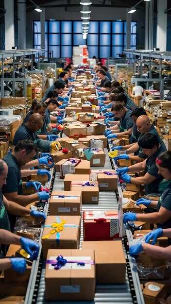
Start with a clear network design: place three micro-fulfillment centers within 2-5 miles of 75–85% of urban orders and implement cross-docking to cut handling cycles by up to 40%. By mapping demand pockets, address near-peak corridors, and setting a 30-minute real-time replenishment window, you reduce movements and boost readiness. Use sensors to monitor slot occupancy and product movement, and align with the transportation plan to maintain high productivity.

Three types of micro-fulfillment nodes help you tailor density: compact automated racks in micro-fulfillment centers, dark stores, and flexible pop-ups near transit corridors. To introduce automation, integrate with your WMS and OMS, then deploy sensors on docks and conveyors to keep movement visible in real-time and guard against stockouts.

For a city-scale network, run a ready model that tests problem scenarios: demand spikes, weather disruptions, and materials shortages. A baseline plan with eight-hour pickup windows, address fulfillment, and cross-docking steps can cut transport miles by 25% and boost productivity by 15–20% within the first quarter of operation. Use real-time dashboards to monitor movement across hubs and fleets, and adjust materials flows to prevent bottlenecks.

へ maintain throughput, establish a real-time data loop across sites. Install sensors on inbound materials and outbound packages to catch temperature, humidity, and tamper events; this helps you address issues before customers notice. Use bikes for the last mile in dense blocks where curb space is tight; combined with dynamic クロスドッキング そして movement tracking, you shave minutes from each delivery and raise on-time rates to 95% or higher.

Next steps: address demand signals with a pilot near a metro center, then introduce a phased expansion plan that integrates with supplier calendars and transport providers. Track types of orders (bulk materials vs. fast-moving SKUs) and tune stock allocations to maximize productivity. Set a ready-to-ship standard at each node and build a movement map that shows where real-time updates flow. Additional improvements come from continuous feedback and tighter materials coordination.

Practical steps for building an agile micro-fulfillment network

Start with a tightly scoped pilot: operate three micro-fulfillment centers in dense metro clusters to deliver a 15–30 minute SLA for a curated grocery basket of 120–150 items. This accelerated rollout demonstrates the method and creates a clear path to scale.

Decide the location mix by analyzing order density, delivery windows, and distance to customers; set decision-making criteria, success metrics, and go/no-go thresholds.

Explore variants of fulfillment models: dark stores, in-store micro-fulfillment, and mobile hubs; these variants influence capital needs and speed to market, and these solutions help teams compare options.

Automating high-volume segments with robotics where ROI is favorable; for other items, rely on skilled people in a hybrid model. The approach continues to scale and makes strongpoints in accuracy and speed.

Streamlined workflows: implement batch picking, zone-based assignment, and put-to-light or pick-to-light where feasible; ensure picked items are placed in a dedicated bag or basket to simplify packing.

Facilitate fast decision-making with real-time dashboards that surface key signals: order volume, item variants, and stock levels; look at data to decide whether to automate more or re-route capacity.

Alternative plans: if a given site cannot host automated equipment, choose an alternative layout or partner for co-located fulfillment; depending on space and ceiling height, scale up gradually. The team chooses the path that best fits local demand.

People-centric design: train staff to operate automation, maintain equipment, and handle exceptions; this reduces turnover and accelerated learning; automation continues to support people.

Race to serve customers: in grocery markets, every minute shaved from order-to-delivery reduces cart abandonment; measure order accuracy, pick error rates, and delivery SLA to win the race.

Offered services expansion: offer same-day, curbside, and locker pickup; align on a consistent service catalog that customers see as a single, dependable experience.

Possible gains come from disciplined capex versus opex checks, ensuring the chosen model aligns with long-term growth.

Define Target Delivery Windows and Zone Coverage for Each MFC

Set target delivery windows per MFC by density tier: 15–20 minutes for high-density urban hubs, 25–40 minutes for regional hubs, and 60–90 minutes for rural zones. These windows should be grounded in real-world routing data and verified with recent pilot results to ensure feasibility under typical traffic and weather conditions. This approach does not require sweeping changes to existing systems, but it does demand disciplined data governance.

Define zone coverage using mile-based radii and road isochrones: urban coverage within a 5 mile radius, suburban coverage up to 15 miles, and rural coverage beyond 15 up to 25 miles. Map distance, travel time, and lane density to avoid excessive overlap and minimize complexity.

Position regional hubs to maximize coverage of highest-demand variants, and use smaller, fully dedicated MFCs near dense neighborhoods to handle fresh SKU variants. This setup reduces back-and-forth trips and lowers last-mile friction.

Use LRPS as a planning metric: LRPS equals expected orders per hour per site, which helps quantify capacity about each MFC. Set targets to sustain the windows and limit travel distance while maintaining long-term resilience. Monitor the number of instances where targets are missed and adjust the number of hubs accordingly.

Data inputs and benchmarking: density, product variants, and order frequency drive boundary setting. Leverage statista data to benchmark density patterns in europe and translate them into regional hub strategies. Use recent demand signals to adjust targets and forecast scenarios.

Operational steps: determine demand by region, set windows, optimize number of MFCs, and map coverage to ensure full regional reach. Account for rural coverage, seasonal variance, and urban growth to keep the plan fresh and adaptable. Start with a conservative LRPS and refine as you validate with real-world results.

Monitoring and metrics: track on-time rate, average miles per delivery, total distance traveled, zone coverage percent, hub utilization, and fresh inventory turnover. Use these metrics to identify bottlenecks and reallocate density to maintain instantly reliable service across all zones.

Select Micro-Fulfillment Locations: Demand Density, Real Estate, and Accessibility

Target high-density demand zones within 3 miles of core customers and validate with a numerical model that scores demand density, real estate cost, and accessibility. The same model aids determining site rankings and informs a portfolio of 4–6 locations in metropolitan markets, enabling rapid expansion while maximizing market share. This approach is very data-driven and fulfilling because it ties productivity to pinpointed sites rather than generic strategies.

Real estate decisions hinge on available spaces that can meet rmls requirements and dock access. Apply a strict cost-per-square-foot rubric while comparing spaces manually to verify fit, including ceiling height, column spacing, and clearance for pallets storing various products. Prioritize spaces within 0.5–2 miles of arterial routes and with at least 2 docks to support next-day or next-shift handoffs, reducing bottlenecks and improving productivity.

Accessibility matters: align MFCs with smart route optimization to minimize last-mile times without sacrificing resilience. Use route-planning systems that factor traffic patterns, dock schedules, and cross-dock handoffs, enabling orders to move directly from pick to pack to ship. This approach supports a scalable network that can route orders from rmls to final destinations efficiently.

Adopt a portfolio across industries and various product families to maximize coverage: electronics, fashion, groceries, and household goods. The model weighting can reflect product characteristics, such as high-velocity SKUs and high-turnover lines; by applying this framework, teams can achieve faster fulfillment and stronger customer satisfaction. theyve achieved measurable gains in throughput and market responsiveness across multiple markets.

Next steps: map demand, identify top 3–5 clusters, and run a pilot with 1–2 MFCs to validate the scoring rubric. In the next phase, collect performance data and adjust the model accordingly. Use what you learn to refine the model and expand the rmls network, taking advantage of available spaces and real-time route insights. The result: a smart, scalable network that enables fast delivery, making the most of a well-chosen location portfolio and driving market share growth.

Model Inventory and Capacity: SKU Mix, Safety Stock, and Rebalancing Rules

Adopt velocity-based SKU mix and automated rebalancing to minimize distance to consumers and maximize on-time delivery across the network.

1. SKU Mix and Zoning
   • Segment SKUs into A (fast movers), B (mid movers), and C (slow movers) using 2- to 4-week demand history and channel signals from omnichannel orders.
   • Target shares: A items ≈ 20% of SKUs delivering 60–70% of volume; B items ≈ 30% delivering 25–30%; C items ≈ 50% delivering 5–15%. Keep the core A set in every warehouse to address point demand while placing B/C items to balance workload across warehouses.
   • For boysen-branded SKUs, designate them as A items if inbound reliability is high; otherwise place them closer to high-demand points to reduce costly inbound trips.
   • Allocate SKUs by geography: denser markets maintain larger cores of fast movers; distant markets carry more niche SKUs to provide assortment without overloading each center.
   • Consider wholesale and direct-to-consumer mixes in the same SKU family to avoid conflicts; align stocking with expected cross-channel returns to keep experience consistent for consumers.
2. Safety Stock and Demand Variability
   • Target service levels by item tier: fast movers get 95%+ coverage for standard 2–3 day inbound lead times; slower movers use 90% coverage with higher variability allowances.
   • Safety stock per SKU uses demand variability during lead time. A practical rule: safety stock ≈ z * σ_DL, where z is the standard normal quantile for the desired service (1.65 for 95%), and σ_DL is the standard deviation of demand over the lead time.
   • Fast movers typically need 3–5 days of average daily usage in stock; seasonal or high-variance SKUs need 7–14 days to buffer promotions or demand spikes.
   • For inventory that handles a return-heavy cycle, add a small buffer dedicated to returns flow to avoid skewing fresh stock levels.
   • In practice, link inbound reliability with safety stock: if inbound on-time performance drops, raise safety stock for affected SKUs to sustain experience.
   • Address product families with low variability using lighter safety stock; for high-variance items, push more frequent monitoring and dynamic adjustment.
3. Rebalancing Rules
   • Run automatic repositioning nightly to keep SKU mix aligned with demand signals, distance to demand points, and returns patterns.
   • Triggers: velocity drift > 15% in a center, projected stock-out risk > 5%, or a shift in return rate that changes replenishment needs.
   • Thresholds avoid thrashing: limit movements to 5–10% of stock value per cycle; prioritize high-velocity SKUs that affect service levels.
   • Distance-driven placement: reallocate SKUs to warehouses within 60–120 km of demand clusters to shorten delivery paths and improve experience.
   • Address omnichannel priorities by keeping a balanced mix at each point in the network, ensuring that online orders, in-store pickup, and wholesale orders receive consistent handling.
4. Inbound and Capacity Alignment
   • Coordinate inbound flows with center capacity: estimate weekly inbound volumes and adjust order windows to prevent overloads in warehousing teams.
   • Use cross-docking where possible to accelerate inbound-to-outbound cycles, reducing handling time and labor costs.
   • Specific item classes like Boysen SKUs may require tighter inbound scheduling if a single supplier handles an important portion of volume; align with wholesale partners to stabilize inbound cadence.
   • Keep buffers at strategic nodes to absorb supplier variability without affecting service levels for consumers.
5. Technologies and Automation
   • Implement inventory optimization engines, WMS, OMS, and TMS that address network-wide SKU mix, safety stock, and rebalancing rules automatically.
   • Use analytics to map distance to demand points and to identify the best warehouse for each SKU daily, which reduces labor intensity and accelerates fulfillment.
   • Address data quality gaps by integrating inbound, returns, and movement data into a single view; provide staff with actionable recommendations rather than raw signals.
   • Provide real-time visibility for managers to intervene when exceptions occur, and to verify that automated decisions align with operational constraints.
6. Metrics, Labor, and Governance
   • Track fill rate per SKU, stock-out rate by center, and order cycle time across channels to measure SKU mix effectiveness and rebalancing impact.
   • Monitor inventory turns, distance traveled per order, and cost per fulfilled order to quantify efficiency gains from the model.
   • Staffing needs vary by center; allocate dedicated personnel to supervise automation, adjust safety stock, and approve rebalancing actions to prevent bottlenecks.
   • Address returns flow separately to ensure it does not destabilize stock levels or distort mix decisions; a disciplined return handling process maintains accuracy across warehouses.

Optimize Last-Mile Routing and Replenishment: Frequency, Consolidation, and Transit Time

Adopt a fixed nightly replenishment window at each micro-fulfilment center to keep fresh stock covered and prevent stockouts, delivering faster restocks for the morning wave.

Analytics-driven routing enables consolidation: build a zone-based last-mile plan that groups orders within a 5–15 km radius where viable, reducing trips and transport cost, and improving service levels across the network.

Determine a consolidation threshold by considering demand levels and seasonality. If forecasted demand in a 60–90 minute window yields at least 20 orders across 4 SKUs, combine into a single run; otherwise dispatch smaller, more frequent trips to maintain freshness and speed.

Transit-time optimization relies on flink-powered streaming analytics to update routes in seconds as traffic shifts. Aim to keep each stop engagement under about 60 seconds to preserve speeds, and target a 10–20% reduction in total transit time versus uncoordinated routing.

Located in sprawling metro areas, distribute micro-fulfilment nodes to shorten covered distances and accelerate pickups, which supports earlier deliveries and steadier replenishment cycles across zones that matter most to customers.

Measure success with analytics on on-time deliveries, fill rate, and cadence of replenishment, and evolve the model year over year. Track cost per fulfilled order to ensure consolidations save money, and identify which combinations of frequency and consolidation yield the strongest returns.heres the practical checklist to start, including a defined cadence, consolidation thresholds, and real-time routing signals (источник) agatz.

Evaluate Costs and Financing Paths: Capex vs Opex, Leasing, and Partnerships

Choose a blended Capex-OpEx plan paired with leasing and partnerships to keep cash flow predictable while maintaining adaptability. Start pilots in untapped zones using robotics applications and modular warehousing equipment; let the data show measurable ROI as volumes grow. Use a clrp framework to align funding with expected results and to keep the plan transparent for stakeholders.

Capex path emphasizes owning high-utility equipment when volumes justify it, including robotics applications and conveyors. Typical upfront ranges: robotics modules 150k–350k per unit; automated storage and retrieval systems 200k–500k; software integration 30k–60k. Annual maintenance and updates run 5–8% of capex, while depreciation spreads cost over 5–7 years. The upside: lower per-unit cost over time and direct control of uptime, with results based budgeting tied to throughput and accuracy.

Opex path and leasing offer flexibility to adapt as shopper demand evolves. Opt for pay-as-you-go robotics services or vendor-managed equipment with 3–5 year terms and typical rates of 6–9% APR. Leasing minimizes upfront cash while maintaining near-term capacity to scale, and service contracts cover software updates, spare parts, and remote monitoring for warehousing and distribution. In europe, providers offer structured leases with flexible end-of-term options, enabling fast experimentation without tying up capital.

Partnerships unlock untapped potential by sharing capex across retailers, landlords, and last-mile operators. Co-investments reduce hurdle barriers and expand the supply of suitable space, especially in zones close to shoppers. Revenue-sharing or operating contracts tie incentives to shopper outcomes such as faster delivery, higher order accuracy, and lower returns, delivering directly measurable results. Experts in leading markets note that particular arrangements can accelerate scale while preserving capital flexibility.

Decision framework: build a zone-based budget and a clrp-led model to compare capex, opex, leasing, and partnerships. Run sensitivity analyses on rate fluctuations, utilization, and demand growth to identify high-probability paths. Define measurable metrics: cycle time, cost per parcel, uptime, energy use, and customer satisfaction scores to show progress. Ensure adaptability to evolve with supply chain changes and become nimble across regions, especially in europe, where rate structures and partnerships vary by market. The goal remains to deliver shopper-centric speed with sustainable unit economics and clear, externally verifiable results based on data.